Tau-U
Parker, Vannest, Davis, and Sauber (2011) proposed Tau-U as an effect size measure for use in single-case designs that exhibit baseline trend. In their original paper, they actually conceptualize Tau-U as a family of four distinct indices, distinguished by a) whether the index includes an adjustment for the presence of baseline trend and b) whether the index incorporates information about trend during the intervention phase. However, in subsequent presentations the authors seem to have focused exclusively on the index that adjusts for baseline trend but not for intervention phase trend, and so I’ll do the same here. (This version is also the one available in the web-tool at singlecaseresearch.org.)
Tau-U is an elaboration on their previously proposed effect sizes NAP and Tau, which do not account for baseline trends. The index is calculated as follows. Suppose that we have data from A and B phases from a single case, where the baseline phase has \(m\) observations and treatment phase has \(n\) observations. Let \(y^A_1,...,y^A_m\) denote the baseline phase data and \(y^B_1,...,y^B_n\) denote the treatment phase data. Tau-U is then calculated as
\[ \text{Tau-U} = \frac{S_P - S_B}{mn} \]
where \(S_P\) is Kendall’s S statistic calculated for the comparison between phases and \(S_B\) is Kendall’s S statistic calculated on the baseline trend. More precisely,
\[ \begin{aligned} S_P &= \sum_{i=1}^m \sum_{j=1}^n \left[I\left(y^B_j > y^A_i\right) - I\left(y^B_j < y^A_i\right)\right] \\ S_B &= \sum_{i=1}^{m - 1} \sum_{j = i + 1}^m \left[I\left(y^A_j > y^A_i\right) - I\left(y^A_j < y^A_i\right)\right]. \end{aligned} \]
Note that the first term in Tau-U is equivalent to \(\text{Tau} = S_P / (m n)\), which in turn is a re-scaling of NAP. The second term is related to the rank-correlation between the measurement occasions and outcomes in the baseline phase. Subtracting the second from the first thus adjusts for baseline trend, in the sense that more pronounced baseline trends will lead to smaller values of Tau-U. But looking at the measure a bit more deeply, it has some very odd features. In this post, I’ll show that the distribution of Tau-U is sensitive to the number of observations in each phase.
Sample size sensitivity
Consider first the logical range of Tau-U. The minimum and maximum possible values of \(S_P\) are \(-m n\) and \(m n\); the minimum and maximum of \(S_B\) are \(-m (m-1) / 2\) and \(m (m - 1) / 2\). Consequently, the logical range of Tau-U is from \(-(2n + m - 1) / (2n)\) to \((2n + m - 1) / (2n)\). If the treatment phase is quite long compared to the baseline phase, then this range will be close to [-1, 1]. On the other hand, in a study with a baseline that is twice as long as the treatment phase, the range of Tau-U will be closer to [-2, 2]. That’s a very odd property.
The average magnitude of Tau-U is similarly influenced by the lengths of each phase. To see this, it’s helpful to think first about its target parameter–the quantity that is estimated when calculating Tau-U based on a sample of data. Since Tau-U is not defined in parametric terms, I will assume that the Tau-U statistic is an unbiased estimator of its target parameter \(\tau_U = \text{E}\left(\text{Tau-U}\right)\). It follows that
\[ \tau_U = \tau_P - \frac{m - 1}{2n} \tau_B, \]
where \(\tau_P\) is Kendall’s rank correlation between the outcomes and an indicator for the treatment phase and \(\tau_B\) is Kendall’s rank correlation between the measurement occasions and outcomes during baseline:
\[ \begin{aligned} \tau_P &= \frac{1}{mn}\sum_{i=1}^m \sum_{j=1}^n \left[\text{Pr}\left(Y^B_j > Y^A_i\right) - \text{Pr}\left(Y^B_j < Y^A_i\right)\right] \\ \tau_B &= \frac{2}{m(m-1)} \sum_{i=1}^{m - 1} \sum_{j = i + 1}^m \left[\text{Pr}\left(Y^A_j > Y^A_i\right) - \text{Pr}\left(Y^A_j < Y^A_i\right)\right]. \end{aligned} \]
Now consider a positive a baseline trend, so that \(\tau_B > 0\), and assume that \(\tau_P\) is constant. A longer baseline phase will then lead to smaller values of Tau-U (on average), while a longer treatment phase will lead to larger values of Tau-U (on average). Again, that’s really weird. This is not a good feature for an effect size measure because it means that Tau-U values from different cases are only on the same scale if the cases have identical baseline and treatment phase lengths. In a multiple baseline study, each case is necessarily observed for a different number of occasions in baseline (otherwise it wouldn’t be a multiple baseline). Thus, it seems inadvisable to use Tau-U to quantify the magnitude of treatment effects in a multiple baseline study.
Sensitivity under a parametric model
Things may be different if we allow for the magnitude of \(\tau_P\) to change along with the sample size. Such would be the case under a model where the intervention phase also exhibits a trend. For example, let’s suppose that the outcome follows a linear model with a non-zero trend and the intervention leads to an immediate shift in the outcome, as in the model:
\[ y_t = \beta_0 + \beta_1 t + \beta_2 I(t > m) + \epsilon_t. \]
For simplicity, I’ll assume that the errors in this model are normally distributed with unit variance. Under this model,
\[ \begin{aligned} \tau_B &= \frac{4}{m (m - 1)} \left[\sum_{i=1}^{m-1} \sum_{j=i+1}^m \Phi\left[\beta_1\left(j - i\right) / \sqrt{2}\right]\right] - 1, \\ \tau_P &= \frac{2}{m n} \left[\sum_{i=1}^m \sum_{j=1}^n \Phi\left[\left(\beta_1 (m + j - i) + \beta_2\right) / \sqrt{2}\right]\right] - 1, \end{aligned} \]
where \(\Phi()\) is the standard normal cumulative distribution function. I can use the above formulas to calculate the average value of Tau-U for various degrees of baseline trend \((\beta_1)\), level shift \((\beta_2)\), and phase lengths \((m,n)\).
E_TauU <- function(b1, b2, m, n) {
  tau_B <- sum(sapply(1:(m - 1), function(i)
    sum(pnorm(b1 * ((i+1):m - i) / sqrt(2))))) * 4 / (m * (m - 1)) - 1
  tau_P <- sum(sapply(1:m, function(i)
    sum(pnorm((b1 * (m + 1:n - i) + b2) / sqrt(2))))) * 2 / (m * n) - 1
  tau_P - tau_B * (m - 1) / (2 * n)
}

library(dplyr)
library(tidyr)
b1 <- c(-0.2, -0.1, 0, 0.1, 0.2)
b2 <- c(0, 0.5, 1.0, 2.0)
m <- c(5, 10, 15, 20)
n <- 5:20

expand.grid(b1 = b1, b2 = b2, m = m, n = n) %>%
  group_by(b1, b2, m, n) %>%
  mutate(TauU = E_TauU(b1, b2, m, n)) ->
  TauU_values
ex <- filter(TauU_values, b1 == -0.2 & b2 == 0)


library(ggplot2)
ggplot(TauU_values, aes(n, TauU, color = factor(m))) +
  facet_grid(b1 ~ b2, labeller = "label_both") +
  geom_line() +
  labs(y = "Expected magnitude of Tau-U", color = "m") +
  theme_bw() + theme(legend.position = "bottom")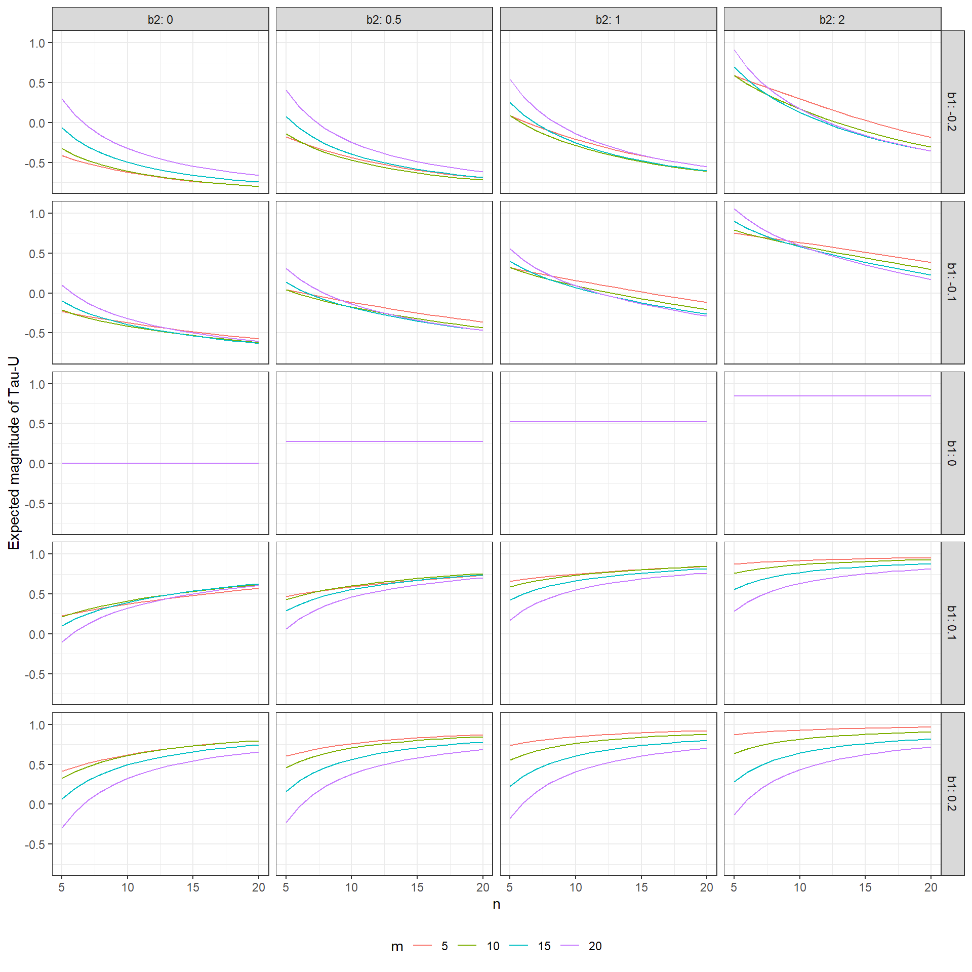
In the figure above, each plot corresponds to a different value of the baseline slope (\(\beta_1\), ranging from -0.2 in the top row to 0.2 in the bottom row) and treatment shift (\(\beta_2\), ranging from 0 in the first column to 2 in the last column). Within each plot, the x axis corresponds to treatment phase length and the different lines correspond to different baseline phase lengths. The thing to note is that, when the baseline slope is non-zero, the expected value of Tau-U ranges quite widely within each plot, depending on the values of \(m\) and \(n\). For example, when \(\beta_2 = 0\) (in the first column), the data follow a simple linear trend with no shift. If the slope of the trend is equal to -0.2 (the first row), then the expected magnitude of Tau-U ranges from -0.8 to 0.3 depending on the phase lengths, which is quite a wide range.
Generally, the degree of sample size sensitivity depends on the absolute magnitude of the baseline slope, with steeper slopes leading to increased sensitivity. For steeper values of slope, it appears that the degree to which the measure is affected by sample size even swamps the degree to which the measure is sensitive to the magnitude of the treatment effect. Very peculiar.
A final thought
Of course, these results are contingent on the particular model under which I derived the expected magnitude of Tau-U. If the data followed some other model, such as a log-linear model with Poisson-distributed outcomes, then the behavior described above might change. Still, I think all of this raises the reasonable question: under what model (i.e., what sort of patterns of baseline trend, what sort of patterns of response to the intervention) does Tau-U provide a meaningful effect size measure that clearly quantifies the magnitude of treatment effects without being strongly affected by phase lengths? Unless and until such a model can be identified, I would be wary of interpreting Tau-U as a measure of treatment effect magnitude.