ARPobservation: Basic use

Simulating behavior streams

Behavior streams are simulated according to an equilibrium alternating renewal process, which involves the following assumptions.

1. Each instance of a behavior, termed an event, lasts a random amount of time, drawn from a specified distribution F_mu with mean mu.

2. The length of time in between instances of behavior, termed the interim time, also lasts a random amount of time, drawn from a specified distribution F_lambda with mean lambda.

3. All events and interim times are mutually independent.

4. The entire process is in equilibrium.

The function r_behavior_stream generates random behavior streams. As an initial example, suppose that both the events and the interim times are exponentially distributed, that events last on average 10 seconds, and that the average interim time is 30 seconds. Also suppose that the behavior stream is observed for 300 seconds. The following code will simulate a behavior stream with these parameters:

library(ARPobservation)
set.seed(8)              # for reproducibility

r_behavior_stream(n = 1, mu = 10, lambda = 30, F_event = F_exp(), F_interim = F_exp(), stream_length = 300)

## $stream_length
## [1] 300
## 
## $b_streams
## $b_streams[[1]]
## $b_streams[[1]]$start_state
## [1] 0
## 
## $b_streams[[1]]$b_stream
##  [1]  61.46643  67.45959 117.53097 120.56840 175.94950 185.74134 265.04376
##  [8] 269.42231 276.13827 284.70467 286.36179 290.82906
## 
## 
## 
## attr(,"class")
## [1] "behavior_stream"

The function returns an object of class behavior_stream, which isn’t terribly nice to look at. The first characteristic of the object is stream_length, which just reports back how long the behavior stream is. The second characteristic is b_streams, a list containing one or more simulated behavior streams. Each behavior stream is also a list. The first element indicate the initial state of the stream, so start_state =0 means that the behavior was not occuring when observation began. The second element is a vector of transition times. The first entry in the vector indicates that the first event began at time 61.47; the following entry indicates that the first event ended (and the next interim time began) at time 67.46. Similarly, the second event began at time 117.53 and ended at time 120.57.

The argument n controls the number of simulated behavior streams returned:

r_behavior_stream(n = 3, mu = 10, lambda = 30, F_event = F_exp(), F_interim = F_exp(), stream_length = 300)

## $stream_length
## [1] 300
## 
## $b_streams
## $b_streams[[1]]
## $b_streams[[1]]$start_state
## [1] 1
## 
## $b_streams[[1]]$b_stream
##  [1]   8.480116  34.311542  43.069956  49.912461  50.087867  85.046893
##  [7] 103.030351 116.377965 117.101992 140.227289 161.762642 180.640609
## [13] 196.060432 201.493182 212.232970 236.486373 238.432946 276.824019
## 
## 
## $b_streams[[2]]
## $b_streams[[2]]$start_state
## [1] 0
## 
## $b_streams[[2]]$b_stream
##  [1]   6.702804  23.820354  26.087981  33.461543  62.786605  74.705604
##  [7] 163.806646 164.761520 271.270557 283.207882 286.136103 297.587748
## 
## 
## $b_streams[[3]]
## $b_streams[[3]]$start_state
## [1] 0
## 
## $b_streams[[3]]$b_stream
##  [1] 196.4605 203.7452 237.9514 245.2451 246.2089 254.6313 256.6439 258.5644
##  [9] 262.1140 265.3249 283.9702 298.7830
## 
## 
## 
## attr(,"class")
## [1] "behavior_stream"

Note that now b_streams is a list with three entries, each of which contains a start_state and a b_stream.

Most of the time, you won’t need to look at the simulated behavior streams directly. Instead, you’ll just simulate a bunch of streams and store them for later analysis. Let’s store 10 simulated behavior streams in an object called BS10:

BS10 <- r_behavior_stream(n = 10, mu = 10, lambda = 30, F_event = F_exp(), F_interim = F_exp(), stream_length = 300)

Applying observation procedures

Several different functions are available to turn the behavior_stream object into familiar types of behavioral observation data. For example, the continuous recording procedure (CDR) involves summarizing the behavior stream by the overall proportion of observation time during which events occur. This can be accomplished by feeding BS into the function continuous_duration_recording:

continuous_duration_recording(BS10)

##  [1] 0.1680877 0.4426930 0.1290537 0.3506492 0.2372437 0.3568621 0.2897521
##  [8] 0.2570101 0.1704727 0.2968024

The function returns a vector containing one number per simulated behavior stream. As expected all of the numbers are proportions between 0 and 1.

More interesting is to simulate many more behavior streams, apply CDR, and calculate the mean and variance of the results or plot them in a histogram:

BS_lots <- r_behavior_stream(n = 10000, mu = 10, lambda = 30, F_event = F_exp(), F_interim = F_exp(), stream_length = 300)
CDR <- continuous_duration_recording(BS_lots)
c(mean = mean(CDR), var = var(CDR))

##        mean         var 
## 0.250140703 0.009567949

hist(CDR)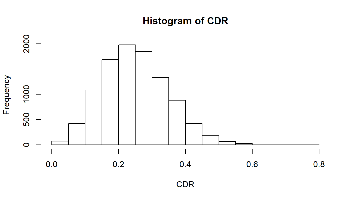

Another well-known recording procedure is partial interval recording (PIR), which involves dividing the observation session into short intervals, then scoring each interval according to whether or not the behavior occurs at any point during the interval. The function interval_recording applies partial interval recording (or the closely related procedure of whole interval recording) to a set of simulated behavior streams. Suppose that the observer uses 20 s intervals, back-to-back for 300 s, for a total of 15 intervals. This procedure can be applied to the simulated behavior streams using

interval_recording(BS10, interval_length = 20, summarize = FALSE)

##       [,1] [,2] [,3] [,4] [,5] [,6] [,7] [,8] [,9] [,10]
##  [1,]    1    0    1    0    1    1    0    0    0     1
##  [2,]    0    0    0    0    1    1    1    1    1     1
##  [3,]    1    1    1    1    1    1    1    1    1     1
##  [4,]    0    1    1    0    1    1    0    0    1     1
##  [5,]    0    1    0    1    0    1    1    0    1     0
##  [6,]    0    1    0    1    0    1    1    1    0     0
##  [7,]    0    1    0    1    0    1    1    1    0     0
##  [8,]    1    1    0    0    1    1    1    1    0     0
##  [9,]    0    1    0    1    0    1    0    1    0     0
## [10,]    0    0    1    1    0    1    1    1    1     0
## [11,]    1    0    0    1    0    1    1    1    0     1
## [12,]    1    1    1    1    0    1    1    1    1     1
## [13,]    1    1    0    1    0    1    1    1    0     1
## [14,]    1    1    1    1    1    1    1    0    1     0
## [15,]    1    1    1    1    1    1    0    1    0     1

Since summarize is set to false, the function returns a 15 by 10 matrix, with one column for each behavior stream. Each column contains one entry for each interval, equal to one if any behavior occured during that interval (and zero otherwise). Typically, PIR data is summarized by calculating the proportion of intervals across the entire observation session. The summary proportion can be calculated automatically by setting the option summarize = TRUE.

interval_recording(BS10, interval_length = 20, summarize = TRUE)

##  [1] 0.5333333 0.7333333 0.4666667 0.7333333 0.4666667 1.0000000 0.7333333
##  [8] 0.7333333 0.4666667 0.5333333

colMeans(interval_recording(BS10, interval_length = 20, summarize = FALSE)) # compare to summarized results

##  [1] 0.5333333 0.7333333 0.4666667 0.7333333 0.4666667 1.0000000 0.7333333
##  [8] 0.7333333 0.4666667 0.5333333

Sometimes, the PIR procedure is used with a short amount of time in between each interval, which allows the observer to record data or notes. Typical use might involve 15 s intervals of active observation, each followed by 5 s of rest time. This procedure can be applied using the rest_proportion option. Since 5 s is 25% of the full interval length, the rest proportion is 0.25.

interval_recording(BS10, interval_length = 20, rest_length = 5, summarize = TRUE)

##  [1] 0.4000000 0.7333333 0.4000000 0.6000000 0.4666667 0.8666667 0.5333333
##  [8] 0.6666667 0.4000000 0.5333333

The whole interval recording procedure is implemented using interval_recording with partial = FALSE. Two other observation procedures are also available: momentary time recording (a.k.a. momentary time sampling), using the function momentary_time_recording, and event counting, using event_counting. See the documentation for these functions for usage and examples.

Finally, a convenience function is available to apply multiple observation procedures to the same set of simulated behavior streams. Suppose that you want to compare the data generated by CDR with the data generated by PIR with 15 s active intervals and 5 s rest times. This can be accomplished using

reported_observations(BS10, data_types = c("C", "P"), interval_length = 20, rest_length = 5)

##            C         P
## 1  0.1680877 0.4000000
## 2  0.4426930 0.7333333
## 3  0.1290537 0.4000000
## 4  0.3506492 0.6000000
## 5  0.2372437 0.4666667
## 6  0.3568621 0.8666667
## 7  0.2897521 0.5333333
## 8  0.2570101 0.6666667
## 9  0.1704727 0.4000000
## 10 0.2968024 0.5333333

This function returns a data frame with one column for each procedure and one row for each simulated behavior stream. Say that you also want to include data based on momentary time recording, with 20 s in between each moment. Just add an "M" to the list of data types to include:

reported_observations(BS10, data_types = c("C", "M", "P"), interval_length = 20, rest_length = 5)

##            C          M         P
## 1  0.1680877 0.20000000 0.4000000
## 2  0.4426930 0.46666667 0.7333333
## 3  0.1290537 0.06666667 0.4000000
## 4  0.3506492 0.40000000 0.6000000
## 5  0.2372437 0.26666667 0.4666667
## 6  0.3568621 0.40000000 0.8666667
## 7  0.2897521 0.26666667 0.5333333
## 8  0.2570101 0.20000000 0.6666667
## 9  0.1704727 0.06666667 0.4000000
## 10 0.2968024 0.20000000 0.5333333