Standard errors and confidence intervals for NAP

Other standard error estimators

Because an equivalent effect size measure is used in other contexts like clinical medicine, there has actually been a fair bit of research into better approaches for assessing the uncertainty in NAP. Hanley and McNeil (1982) proposed an estimator for the sampling variance of NAP that is designed for continuous outcome measures, where exact ties are impossible. Modifying it slightly (and in entirely ad hoc fashion) to account for ties, let

\[ \begin{aligned} Q_1 &= \frac{1}{m n^2}\sum_{i=1}^m \left[\sum_{j=1}^n I\left(y^B_j > y^A_i\right) + 0.5 I\left(y^B_j = y^A_i\right)\right]^2 \\ Q_2 &= \frac{1}{m^2 n}\sum_{j=1}^n \left[\sum_{i=1}^m I\left(y^B_j > y^A_i\right) + 0.5 I\left(y^B_j = y^A_i\right)\right]^2. \end{aligned} \]

Then the Hanley-McNeil variance estimator is

\[ V_{HM} = \frac{1}{mn} \left[\text{NAP}\left(1 - \text{NAP}\right) + (n - 1)\left(Q_1 - \text{NAP}^2\right) + (m - 1)\left(Q_2 - \text{NAP}^2\right)\right], \]

with \(\text{SE}_{HM} = \sqrt{V_{HM}}\).

The same authors also propose a different estimator, which is based on the assumption that the outcome data are exponentially distributed. Even though this is a strong and often inappropriate assumption, there is evidence that this estimator works even for other, non-exponential distributions. Newcombe (2006) suggested a further modification of their estimator, and I’ll describe his version. Let \(h = (m + n) / 2 - 1\). Then

\[ V_{New} = \frac{h}{mn} \text{NAP}\left(1 - \text{NAP}\right)\left[\frac{1}{h} + \frac{1 - \text{NAP}}{2 - \text{NAP}} + \frac{\text{NAP}}{1 + \text{NAP}}\right], \]

with \(\text{SE}_{New} = \sqrt{V_{New}}\).

Here are R functions to calculate each of these variance estimators.

V_HM <- function(yA, yB) {
  m <- length(yA)
  n <- length(yB)
  U <- sapply(yB, function(j) (j > yA) + 0.5 * (j == yA))
  t <- sum(U) / (m * n)
  Q1 <- sum(rowSums(U)^2) / (m * n^2)
  Q2 <- sum(colSums(U)^2) / (m^2 * n)
  (t * (1 - t) + (n - 1) * (Q1 - t^2) + (m - 1) * (Q2 - t^2)) / (m * n)
}

V_New <- function(yA, yB) {
  m <- length(yA)
  n <- length(yB)
  t <- NAP(yA, yB)
  h <- (m + n) / 2 - 1
  t * (1 - t) * (1 + h * (1 - t) / (2 - t) + h * t / (1 + t)) / (m * n)
}

sqrt(V_HM(yA, yB))

## [1] 0.03483351

sqrt(V_New(yA, yB))

## [1] 0.04370206

For the worked example dataset from Parker and Vannest, the Newcombe estimator yields a standard error that is about 25% larger than the Hanley-McNeil estimator. Both of these are substantially smaller than the null standard error, which in this example is \(\text{SE}_{null} = 0.129\).

A small simulation

Simulation methods can be used to examine how well these various standard error formulas estimate the actual sampling variation of NAP. For simplicity, I’ll simulate normally distributed data where

\[ Y^A \sim N(0, 1) \qquad \text{and} \qquad Y^B \sim N\left(\sqrt{2}\Phi^{-1}(\theta), 1\right) \]

for varying values of the effect size estimand (\(\theta\)) and a couple of different sample sizes.

sample_NAP <- function(delta, m, n, iterations) {
  NAPs <- replicate(iterations, {
    yA <- rnorm(m)
    yB <- rnorm(n, mean = delta)
    c(NAP = NAP(yA, yB), V_HM = V_HM(yA, yB), V_New = V_New(yA, yB))
  })
  data.frame(sd = sd(NAPs["NAP",]), 
             SE_HM = sqrt(mean(NAPs["V_HM",])), 
             SE_New = sqrt(mean(NAPs["V_New",])))
}

library(dplyr)
library(tidyr)
theta <- seq(0.5, 0.95, 0.05)
m <- c(5, 10, 15, 20, 30)
n <- c(5, 10, 15, 20, 30)

expand.grid(theta = theta, m = m, n = n) %>%
  group_by(theta, m, n) %>% 
  mutate(delta = sqrt(2) * qnorm(theta)) ->
  params 

params %>%
  do(sample_NAP(.$delta, .$m, .$n, iterations = 2000)) %>%
  mutate(se_null = sqrt((m + n + 1) / (12 * m * n))) %>%
  gather("sd","val", sd, SE_HM, SE_New, se_null) ->
  NAP_sim

library(ggplot2)
ggplot(NAP_sim, aes(theta, val, color = sd)) + 
  facet_grid(n ~ m, labeller = "label_both") + 
  geom_line() + 
  theme_bw() + theme(legend.position = "bottom")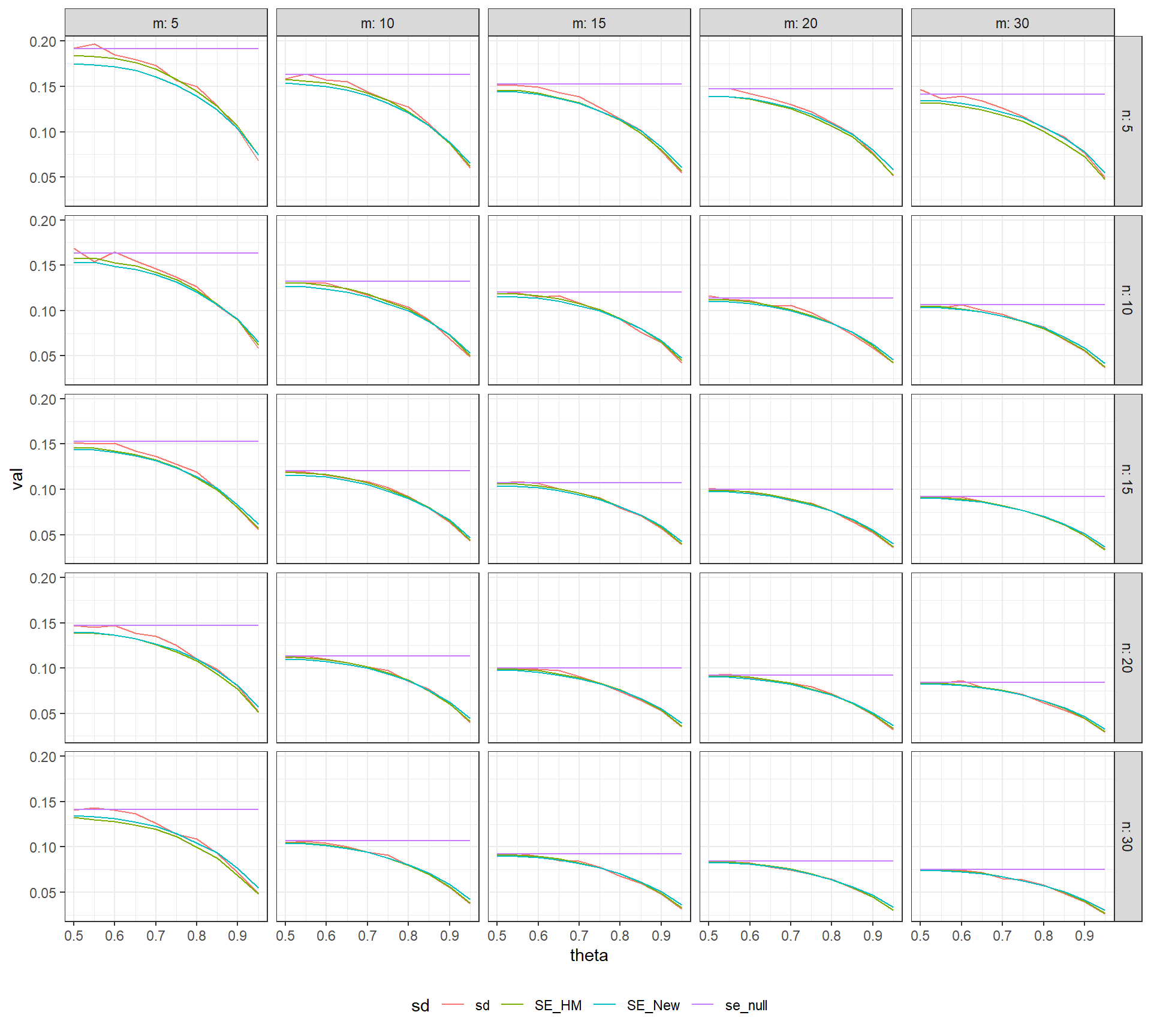

In the above figure, the actual sampling standard deviation of NAP (in red) and the value of \(\text{SE}_{null}\) (in purple) are plotted against the true value of \(\theta\), with separate plots for various combinations of \(m\) and \(n\). The expected value of the standard errors \(\text{SE}_{HM}\) and \(\text{SE}_{New}\) (actually the square root of the expectation of the variance estimators) are depicted in green and blue, respectively. The value of \(\text{SE}_{null}\) agrees with the actual standard error when \(\delta = 0\), but the two diverge when there is a positive treatment effect. It appears that \(\text{SE}_{HM}\) and \(\text{SE}_{New}\) both under-estimate the actual standard error when \(m\) or \(n\) is equal to 5, and over-estimate for the largest values of \(\theta\). However, both of these estimators offer a marked improvement over \(\text{SE}_{null}\).

Other confidence intervals

As I noted above, there has been a fair amount of previous research into how to construct CIs for \(\theta\), the parameter estimated by NAP. As is often the case with these sorts of problems, there are many different methods available, scattered across the literature. Fortunately, there are two (at least) fairly comprehensive simulation studies that compare the performance of various methods under a wide range of conditions. Newcombe (2006) examined a range of methods based on inverting Wald-type test statistics (which give CIs of the form \(\text{estimate} \pm \text{SE} \times z_{\alpha / 2}\), where \(\text{SE}\) is some standard error estimate) and score-based methods (in which the standard error is estimated using the candidate parameter value). Based on an extensive simulation, he suggested a score-based method in which the end-points of the CI are defined the values of \(\theta\) that satisfy:

\[ (\text{NAP} - \theta)^2 = \frac{z^2_{\alpha / 2} h \theta (1 - \theta)}{mn}\left[\frac{1}{h} + \frac{1 - \theta}{2 - \theta} + \frac{\theta}{1 + \theta}\right], \]

where \(h = (m + n) / 2 - 1\). This equation is a fourth-degree polynomial in \(\theta\), easily solved using a numerical root-finding algorithm.

In a different simulation study, Ruscio and Mullen (2012) examined the performance of a selection of different confidence intervals for \(\theta\), including several methods not considered by Newcombe. Among the methods that they examined, they find that the bias-corrected, accelerated (BCa) bootstrap CI performs particularly well (and seems to outperform the score-based CI recommended by Newcombe).

Neither Newcombe (2006) nor Ruscio and Mullen (2012) considered constructing a confidence interval by directly pivoting the Mann-Whitney U test (the same technique used to construct confidence intervals for the Hodges-Lehmann estimator of location shift), although it seems to me that this would be possible and potentially an attractive approach in the context of SCDs. The main caveat is that such a CI would require stronger distributional assumptions than those studied in the simulations, such as that the distributions of \(Y^A\) and \(Y^B\) differ by an additive (or multiplicative) constant. In any case, it seems like it would be worth exploring this approach too.

Another small simulation

Here is an R function for calculating several different CIs for \(\theta\), including the null CI, Wald-type CIs based on \(V_{HM}\) and \(V_{New}\), and the score-type CI recommended by Newcombe (2006). I haven’t programmed the BCa bootstrap because it would take a bit more thought to figure out how to simulate it efficiently.

The following code simulates the coverage rates of nominal 90% CIs based on each of these methods, following the same simulation set-up as above.

NAP_CIs <- function(yA, yB, alpha = .05) {
  m <- length(yA)
  n <- length(yB)
  U <- sapply(yB, function(j) (j > yA) + 0.5 * (j == yA))
  t <- sum(U) / (m * n)
  
  # variance estimators
  V_null <- (m + n + 1) / (12 * m * n)
  
  Q1 <- sum(rowSums(U)^2) / (m * n^2)
  Q2 <- sum(colSums(U)^2) / (m^2 * n)
  V_HM <- (t * (1 - t) + (n - 1) * (Q1 - t^2) + (m - 1) * (Q2 - t^2)) / (m * n)
  
  h <- (m + n) / 2 - 1
  V_New <- t * (1 - t) * (1 + h * (1 - t) / (2 - t) + h * t / (1 + t)) / (m * n)
  
  # Wald-type confidence intervals
  z <- qnorm(1 - alpha / 2)
  SEs <- sqrt(c(null = V_null, HM = V_HM, Newcombe = V_New))
  Wald_lower <- t - z * SEs
  Wald_upper <- t + z * SEs
  
  # score-type confidence interval
  f <- function(x) m * n * (t - x)^2 * (2 - x) * (1 + x) - 
    z^2 * x * (1 - x) * (2 + h + (1 + 2 * h) * x * (1 - x))
  score_lower <- if (t > 0) uniroot(f, c(0, t))$root else 0
  score_upper <- if (t < 1) uniroot(f, c(t, 1))$root else 1
  list(NAP = t, 
       CI = data.frame(lower = c(Wald_lower, score = score_lower), 
                       upper = c(Wald_upper, score = score_upper)))
}

NAP_CIs(yA, yB)

## $NAP
## [1] 0.9636364
## 
## $CI
##              lower     upper
## null     0.7106061 1.2166666
## HM       0.8953639 1.0319088
## Newcombe 0.8779819 1.0492908
## score    0.7499741 0.9950729

sample_CIs <- function(delta, m, n, alpha = .05, iterations) {
  NAPs <- replicate(iterations, {
    yA <- rnorm(m)
    yB <- rnorm(n, mean = delta)
    NAP_CIs(yA, yB, alpha = alpha)
  }, simplify = FALSE)
  theta <- mean(sapply(NAPs, function(x) x$NAP))
  coverage <- rowMeans(sapply(NAPs, function(x) (x$CI$lower < theta) & (theta < x$CI$upper)))
  data.frame(CI = rownames(NAPs[[1]]$CI), coverage = coverage)
}

params %>% 
  do(sample_CIs(delta = .$delta, m = .$m, n = .$n, alpha = .10, iterations = 5000)) ->
  NAP_CI_sim

ggplot(NAP_CI_sim, aes(theta, coverage, color = CI)) + 
  facet_grid(n ~ m, labeller = "label_both", scales = "free_y") + 
  geom_line() + 
  labs(y = "SE") + 
  geom_hline(yintercept=.90, linetype="dashed") +
  theme_bw() + theme(legend.position = "bottom")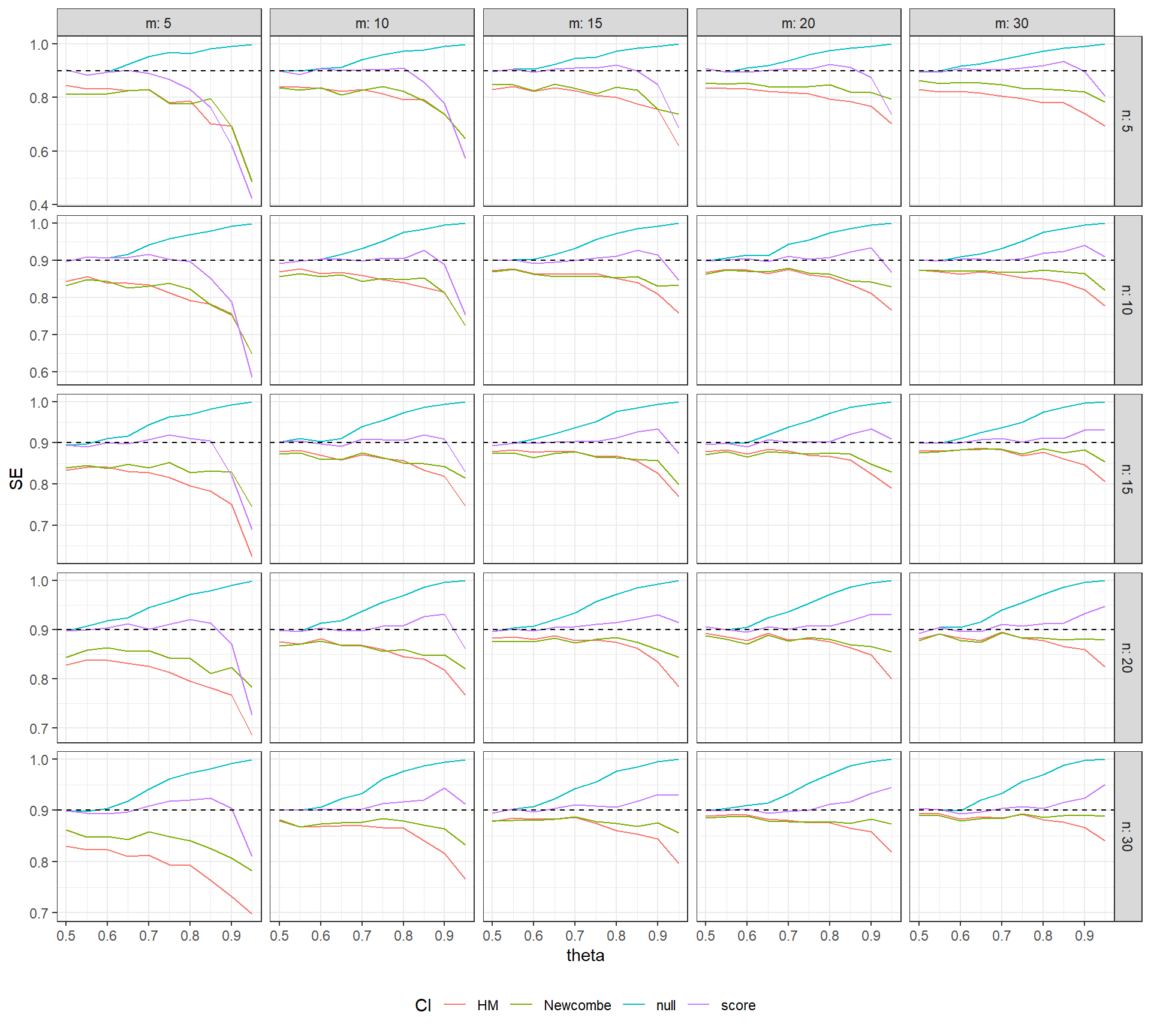

The figure above plots the coverage rates of several different confidence intervals for \(\theta\): the naive CI (in blue), the HM Wald CI (red), the Newcombe Wald CI (green), and the Newcombe score CI (purple). The dashed horizontal line is the nominal coverage rate of 90%. It can be seen that the null CI has the correct coverage only when \(\theta \leq .6\); for larger values of \(\theta\), its coverage becomes too conservative (tending towards 100%). The Wald-type CIs have below-nominal coverage rates, which improve as the sample size in each phase increases but remain too liberal even at the largest sample size considered. Finally, Newcombe’s score CI maintains close-to-nominal coverage over a wider range of \(\theta\) values. Although these CIs have below-nominal coverage for the smallest sample sizes, they generally have good coverage for \(\theta < .9\) and when the sample size in each phase is 10 or more. It is also notable that their coverage rates appear to become more accurate as the sample size in a given group increases, even if the sample size in the other group is fairly small and remains constant.