Variance component estimates in meta-analysis with mis-specified sampling correlation
\[ \def\Pr{{\text{Pr}}} \def\E{{\text{E}}} \def\Var{{\text{Var}}} \def\Cov{{\text{Cov}}} \]
In a recent paper with Beth Tipton, we proposed new working models for meta-analyses involving dependent effect sizes. The central idea of our approach is to use a working model that captures the main features of the effect size data, such as by allowing for both between- and within-study heterogeneity in the true effect sizes (rather than only between-study heterogeneity). Doing so will lead to more precise estimates of overall average effects or, in models that include predictor variables, more precise estimates of meta-regression coefficients. Further, one can combine this working model with robust variance estimation methods to provide protection against the possibility that some of the model’s assumptions could be mis-specified.
In order to estimate these new working models, the analyst must first make some assumption about the degree of correlation between effect size estimates that come from the same sample. In typical applications, it can be difficult to obtain good empirical information about the correlation between effect size estimates, and so it is common to impose some simplifying assumptions and use rough guesses about the degree of correlation. There’s a sense that this might not matter much—particularly because robust variance estimation should protect the inferences if the assumptions about the correlation are wrong. However, I’m still curious about the extent to which these assumptions about the correlation structure matter for anything.
There’s a few reasons to wonder about how much the correlation matters. One is that the analyst might actually care about the variance component estimates from the working model, if they’re substantively interested in the extent of heterogeneity or if they’re trying to make predictions about the distribution of effect sizes that could be expected in a new study. Compared to earlier working models, the variance component estimates of the models that we proposed in the paper seem to be relatively more sensitive to the assumed correlation. Second, one alternative analytic strategy that’s been proposed (and applied) for meta-analysis of dependent effect sizes is to use a multi-level meta-analysis (MLMA) model. The MLMA is a special case of the correlated-and-hierarchical effects model that we described in the paper, the main difference being that MLMA ignores any correlations between effect size estimates (at the level of the sampling errors), or equivalently, assumes that the correlations are all zero. Thus, MLMA is one specific way that this correlation assumption might be mis-specified. There’s some simulation evidence that inferences based on MLMA may be robust (even without using robust variance estimation), but it’s not clear how general this robustness property might be.
In this post, I’m going to look at the implications of using a mis-specified assumption about the sampling correlation for the variance components in the correlated-and-hierarchical effects working model. As in my previous post on weights in multivariate meta-analysis, I’m going to mostly limit consideration to the simple (but important!) case of an intercept-only model, without any further predictors of effect size, to see what can be learned about how the variance components can go wrong.
Mis-specified REML
To figure out what’s going on here, we need to know something about how REML estimators behave under mis-specified models. For starters, I’ll work with a more general case than the CHE model described above. Suppose that we have a vector of multi-variate normal outcomes \(\mathbf{T}_j\) for \(j = 1,...,J\), explained by a set of covariates \(\mathbf{X}_j\), and with true variance-covariance matrix \(\boldsymbol\Phi_j\): \[ \mathbf{T}_j \ \sim \ N\left( \mathbf{X}_j \beta, \boldsymbol\Phi_j \right) \] However, suppose that we posit a variance structure \(\boldsymbol\Omega_j(\boldsymbol\theta)\), which is a function of a \(v\)-dimensional variance component parameter \(\boldsymbol\theta\), and where \(\boldsymbol\Phi_j\) is not necessarily conformable to \(\boldsymbol\Omega_j(\boldsymbol\theta)\). Let \(\mathbf{T}\) and \(\mathbf{X}\) denote the full vector of outcomes and the full (stacked) predictor matrix for \(j = 1,...,J\), and let \(\boldsymbol\Phi\) and \(\boldsymbol\Omega\) denote the corresponding block-diagonal variance-covariance matrices.
We estimate \(\boldsymbol\theta\) by REML, which maximizes the log likelihood \[ 2 l_R(\boldsymbol\theta) = c -\log \left|\boldsymbol\Omega_j(\boldsymbol\theta)\right| - \log \left|\mathbf{X}' \boldsymbol\Omega^{-1}_j(\boldsymbol\theta) \mathbf{X}\right| - \mathbf{T}'\mathbf{Q}(\boldsymbol\theta)\mathbf{T}, \] where \(\mathbf{Q}(\boldsymbol\theta) = \boldsymbol\Omega^{-1}_j(\boldsymbol\theta) - \boldsymbol\Omega^{-1}_j(\boldsymbol\theta) \mathbf{X} \left(\mathbf{X}' \boldsymbol\Omega^{-1}_j(\boldsymbol\theta) \mathbf{X}\right)^{-1} \mathbf{X}'\boldsymbol\Omega^{-1}_j(\boldsymbol\theta)\). Equivalently, the REML estimators solve the score equations \[ \frac{\partial l_R(\boldsymbol\theta)}{\partial \theta_q} = 0, \qquad \text{for} \qquad q = 1,...,v. \]
Under mis-specification, the REML estimators converge (as \(J\) increases) to the values that minimize the Kullback-Liebler divergence between the posited model and the true data-generating process. For the restricted likelihood, the Kullback-Liebler divergence is given by \[ \begin{aligned} \mathcal{KL}(\theta, \theta_0) &= \E\left[l_R(\boldsymbol\Phi) - l_R(\boldsymbol\theta)\right] \\ &= c + \log \left| \boldsymbol\Omega(\boldsymbol\theta) \right| + \log \left| \mathbf{X}'\boldsymbol\Omega^{-1}(\boldsymbol\theta) \mathbf{X} \right| + \text{tr}\left(\mathbf{Q}(\boldsymbol\theta) \boldsymbol\Phi\right), \end{aligned} \] where the expectation in the first line is taken with respect to the true data-generating process and where \(c\) (in the second line) is a constant that does not depend on \(\boldsymbol\theta\).
Back to CHE
Let me now jump back to the special case of the CHE model for a meta-analysis with no predictors. Let \(\tau_*^2\) and \(\omega_*^2\) denote the variance components in the true data-generating process. Let \(\tilde\tau^2\) and \(\tilde\omega^2\) denote the asymptotic limits of the REML estimators under the mis-specified model. In this model, \(\mathbf{X}_j = \mathbf{1}_j\), \[ \begin{aligned} \boldsymbol\Phi_j &= \left(\tau_*^2 + \phi \sigma_j^2\right) \mathbf{1}_j \mathbf{1}_j' + \left(\omega_*^2 + (1 - \phi) \sigma_j^2\right) \mathbf{I}_j \\ \boldsymbol\Omega_j &= \left(\tilde\tau^2 + \rho \sigma_j^2\right) \mathbf{1}_j \mathbf{1}_j' + \left(\tilde\omega^2 + (1 - \rho) \sigma_j^2\right) \mathbf{I}_j \\ \boldsymbol\Omega_j^{-1} &= \frac{1}{\tilde\omega^2 + (1 - \rho)\sigma_j^2}\left[\mathbf{I}_j - \frac{\tilde\tau^2 + \rho \sigma_j^2}{k_j \tilde\tau^2 + k_j \rho \sigma_j^2 + \tilde\omega^2 + (1 - \rho)\sigma_j^2} \mathbf{1}_j \mathbf{1}_j' \right]. \end{aligned} \] Let \(\displaystyle{\tilde{w}_j = \frac{k_j}{k_j \tilde\tau^2 + k_j \rho \sigma_j^2 + \tilde\omega^2 + (1 - \rho)\sigma_j^2}}\) denote the weight assigned to study \(j\) under the mis-specified model, with the total weight denoted as \(\displaystyle{\tilde{W} = \sum_{j=1}^J \tilde{w}_j}\). Similarly, let \(\displaystyle{w^*_j = \frac{k_j}{k_j \tau_*^2 + k_j \phi \sigma_j^2 + \omega_*^2 + (1 - \phi)\sigma_j^2}}\) denote the weight that should be assigned to study \(j\) under the true model. Then we have that \[ \begin{aligned} \text{tr}\left(\mathbf{Q} \boldsymbol\Phi\right) &= \text{tr}\left(\boldsymbol\Omega^{-1} \boldsymbol\Phi\right) - \text{tr}\left[\left(\mathbf{1}'\boldsymbol\Omega^{-1} \mathbf{1}\right)^{-1} \mathbf{1}'\boldsymbol\Omega^{-1} \boldsymbol\Phi \boldsymbol\Omega^{-1} \mathbf{1}\right] \\ &= \sum_{j=1}^J \text{tr}\left(\boldsymbol\Omega^{-1}_j \boldsymbol\Phi_j\right) - \frac{1}{\tilde{W}}\sum_{j=1}^J \mathbf{1}_j'\boldsymbol\Omega^{-1}_j \boldsymbol\Phi_j \boldsymbol\Omega_j^{-1} \mathbf{1}_j \\ &= \sum_{j=1}^J \frac{k_j}{\tilde\omega^2 + (1 - \rho)\sigma_j^2}\left[\tau_*^2 + \omega_*^2 + \sigma_j^2 - \left(\tilde\tau^2 + \rho \sigma_j^2\right) \frac{\tilde{w}_j}{w^*_j}\right] - \frac{1}{\tilde{W}}\sum_{j=1}^J \frac{\tilde{w}_j^2}{w^*_j} \\ &= \sum_{j=1}^J (k_j - 1) \left(\frac{\omega_*^2 + (1 - \phi)\sigma_j^2}{\tilde\omega^2 + (1 - \rho)\sigma_j^2}\right) + \sum_{j=1}^J \frac{\tilde{w}_j}{w_j^*} - \frac{1}{\tilde{W}}\sum_{j=1}^J \frac{\tilde{w}_j^2}{w^*_j}, \end{aligned} \] and \[ \log \left| \boldsymbol\Omega \right| = \sum_{j=1}^J\log \left| \boldsymbol\Omega_j \right| = \sum_{j=1}^J\left[ \left(k_j - 1\right) \log\left(\tilde\omega^2 + (1 - \rho)\sigma_j^2\right) - \log \left(\frac{\tilde{w}_j}{k_j}\right)\right] \] and \[ \log \left|\mathbf{1}'\boldsymbol\Omega^{-1} \mathbf{1}\right| = \log \left(\tilde{W}\right), \] It follows that the REML estimators converge to the values \(\tilde\tau^2\) and \(\tilde\omega^2\) that minimize \[ \begin{aligned} \mathcal{KL}\left(\tilde\tau^2, \tilde\omega^2, \rho, \tau_*^2, \omega_*^2, \phi\right) &= \sum_{j=1}^J (k_j - 1) \left(\frac{\omega_*^2 + (1 - \phi)\sigma_j^2}{\tilde\omega^2 + (1 - \rho)\sigma_j^2}\right) + \sum_{j=1}^J \frac{\tilde{w}_j}{w_j^*} - \frac{1}{\tilde{W}}\sum_{j=1}^J \frac{\tilde{w}_j^2}{w^*_j} \\ & \qquad \qquad + \sum_{j=1}^J\left(k_j - 1\right) \log\left(\tilde\omega^2 + (1 - \rho)\sigma_j^2\right) - \sum_{j=1}^J \log \left(\frac{\tilde{w}_j}{k_j}\right) + \log(\tilde{W}) \end{aligned} \] This is a complicated non-linear objective function, but it can be minimized numerically using standard techniques.
Here are some heatmaps of the function for \(\tau = 0.2\), \(\omega = 0.1\), \(\phi = 0.4\), and some simulated values for \(k_j\) and \(\sigma_j^2\), for three different assumed correlations:
library(tidyverse)
set.seed(20211124)

CHE_KL <- function(to, tau, omega, phi, rho, k_j, sigmasq_j) {

  trs_j <- to[1]^2 + rho * sigmasq_j
  ors_j <- to[2]^2 + (1 - rho) * sigmasq_j
  w_j <- k_j / (k_j * trs_j + ors_j)
  W <- sum(w_j)

  tausq_ps_j <- tau^2 + phi * sigmasq_j
  omegasq_ps_j <- omega^2 + (1 - phi) * sigmasq_j
  wj_star <- k_j / (k_j * tausq_ps_j + omegasq_ps_j)

  A1 <- sum((k_j - 1) * omegasq_ps_j / ors_j)
  A2 <- sum(w_j / wj_star)
  A3 <- sum(w_j^2 / wj_star) / W
  B <- sum((k_j - 1) * log(ors_j) - log(w_j / k_j))
  C <- log(W)

  A1 + A2 - A3 + B + C

}

tau <- 0.2
omega <- 0.1
phi <- 0.4
J <- 20
k_j <- 1 + rpois(J, 5)
sigmasq_j <- 4 / pmax(rgamma(J, 3, scale = 30), 20)


KL_dat <-
  cross_df(list(t = seq(0,0.4,0.01),
                o = seq(0,0.2,0.005),
                rho = c(0, 0.4, 0.8))) %>%
  mutate(
    to = map2(.x = t, .y = o, ~ c(.x, .y)),
    KL = map2_dbl(.x = to, .y = rho, .f = CHE_KL,
                  tau = tau, omega = omega,
                  phi = phi, k_j = k_j, sigmasq_j = sigmasq_j),
    rho = paste("rho ==", rho)
  ) %>%
  group_by(rho)

KL_min <-
  KL_dat %>%
  filter(KL == min(KL))

KL_dat %>%
  mutate(KL = -pmin(0.25, (KL - min(KL)) / (max(KL) - min(KL)))) %>%
ggplot() +
  facet_wrap(~ rho, scales = "free", labeller = "label_parsed") +
  geom_contour_filled(aes(x = t, y = o, z = KL), bins = 30) +
  geom_point(x = tau, y = omega, color = "white", size = 2) +
  geom_point(data = KL_min, aes(x = t, y = o), color = "red", size = 2) +
  theme_minimal() +
  labs(x = expression(tau), y = expression(omega)) +
  scale_x_continuous(expand = c(0,0)) +
  scale_y_continuous(expand = c(0,0)) +
  theme(legend.position = "none")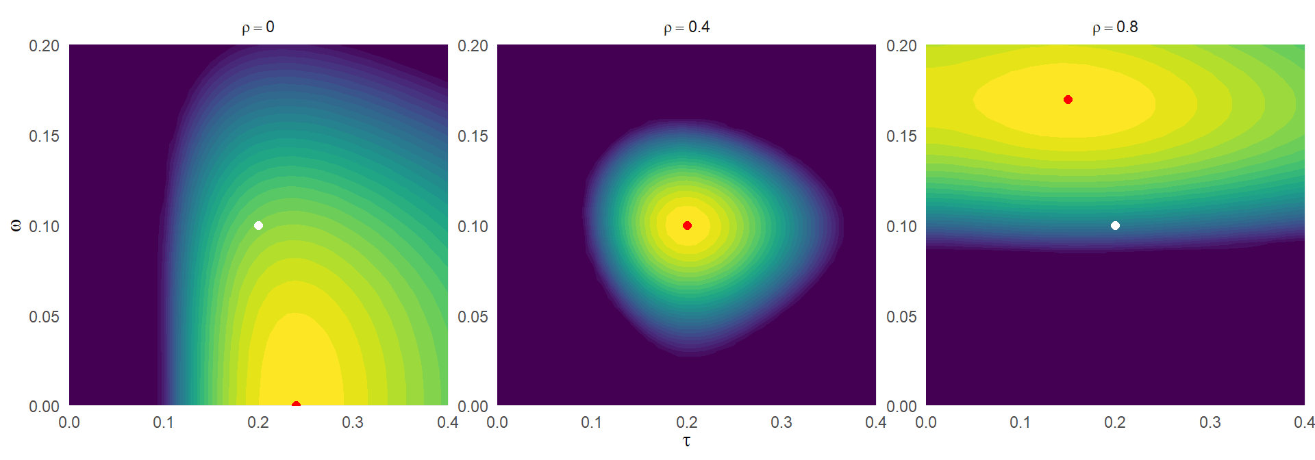
The white points correspond to the true parameter values, while the red points correspond with the values that minimized the K-L divergence. In the middle plot, where \(\rho = 0.4\) corresponds to the true sampling correlation, the function is minimized at the true values of \(\tau\) and \(\omega\). In the left-hand plot, assuming \(\rho = 0.0\) leads to an upwardly biased value of \(\tau\) and a downwardly biased value of \(\omega\). In the right-hand plot, assuming \(\rho = 0.8\) leads to a smaller value of \(\tau\) and a larger value of \(\omega\).
Completely balanced designs
Things simplify considerably in the special case that the sample of studies is completely balanced, such that \(k_1 = k_2 = \cdots = k_J\) and \(\sigma_1^2 = \sigma_2^2 = \cdots = \sigma_J^2\). In such a design, the log-likelihood depends on \(\tau^2\) and \(\omega^2\) only through the quantities \(a = \tau^2 + \rho \sigma^2\) and \(b = \omega^2 + (1 - \rho) \sigma^2\). It follows that \[ l_R\left(\tau^2, \omega^2, \phi\right) = l_R\left(\tilde\tau^2, \tilde\omega^2, \rho\right) \] so long as \[ \begin{aligned} \tau^2 + \phi \sigma^2 &= \tilde\tau^2 + \rho \sigma^2 \\ \omega^2 + (1 - \phi)\sigma^2 &= \tilde\omega^2 + (1 - \rho) \sigma^2. \end{aligned} \] If we assume that \((\rho - \phi)\sigma^2 < \tau^2\) and \((\phi - \rho)\sigma^2 < \omega^2\), then we can set \[ \begin{aligned} \tilde\tau^2 &= \tau^2 - \left(\rho - \phi\right) \sigma^2 \\ \tilde\omega^2 &= \omega^2 + \left(\rho - \phi\right) \sigma^2 \end{aligned} \] and achieve the exact same likelihood.1 Because the Kullback-Liebler divergence is minimized at the log likelihood of the true parameter values, setting \(\tilde\tau^2\) and \(\tilde\omega^2\) equal to the above quantities will also minimize the K-L divergence.
The relationships here are fairly intuitive, I think. When \(\rho\) is an over-estimate of the true correlation \(\phi\), then the between-study variance will be under-estimated and the within-study variance will be over-estimated, each to an extent that depends on a) the difference between \(\rho\) and \(\phi\) and b) the size of the (average) sampling variance. When \(\rho\) is an under-estimate of the true correlation \(\phi\), then the between-study variance will be over-estimated and the within-study variance will be under-estimated, each to an extent that depends on the same components. It’s also rather intriguing to see that the total variance (the sum of \(\tau^2\) and \(\omega^2\)) is totally invariant to \(\rho\) and will be preserved no matter what assumption we make regarding the sample correlation.
In practice, of course, it’s pretty unlikely to have a meta-analytic dataset that is completely balanced. Still, the formulas for this completely balanced case might nonetheless be useful as heuristics for the direction of the biases in the parameter estimates—perhaps even as rough guides for the magnitude of bias that could be expected.
Finding \(\tilde\tau^2\) and \(\tilde\omega^2\) in imbalanced designs
In imbalanced designs, we can find \(\tilde\tau^2\) and \(\tilde\omega^2\) by direct minimization of \(\mathcal{KL}\), given design information \(k_1,...,k_J\) and \(\sigma_1^2,...,\sigma_J^2\); true parameter values \(\tau^2\), \(\omega^2\), \(\phi\); and assumed correlation \(\rho\). The plot below depicts how \(\tilde\tau\), \(\tilde\omega\), and the total SD \(\sqrt{\tilde\tau^2 + \tilde\omega^2}\) change as a function of the assumed correlation \(\rho\), for various levels of true correlation \(\phi\), when the design is imbalanced. As previously, I use \(\tau = 0.2\) and \(\omega = 0.1\).
find_tau_omega <- function(tau, omega, phi, rho, k_j, sigmasq_j) {

  res <- optim(par = c(tau + 0.001, omega + 0.001), fn = CHE_KL,
                tau = tau, omega = omega, phi = phi, rho = rho,
                k_j = k_j, sigmasq_j = sigmasq_j,
                lower = c(0,0), method = "L-BFGS-B")

  data.frame(tau_tilde = res$par[1], omega_tilde = res$par[2])
}

sigmasq_bar <- mean(sigmasq_j)

opt_params <-
  cross_df(list(tau = tau,
                omega = omega,
                phi = seq(0.2,0.8,0.2),
                rho = seq(0,0.95,0.05))) %>%
  mutate(
    res = pmap(., .f = find_tau_omega, k_j = k_j, sigmasq_j = sigmasq_j),
  ) %>%
  unnest(res) %>%
  mutate(
    total_tilde = sqrt(tau_tilde^2 + omega_tilde^2),
    tau_pred = sqrt(pmax(0,tau^2 + (phi - rho) * sigmasq_bar)),
    omega_pred = sqrt(pmax(0, omega^2 - (phi - rho) * sigmasq_bar)),
    total_pred = sqrt(tau_pred^2+ omega_pred^2),
    phi_lab = paste("phi ==", phi)
  )

opt_params %>%
  pivot_longer(c(ends_with("_tilde"), ends_with("_pred")),
               names_to = "q", values_to = "p") %>%
  separate(q, into = c("param","type")) %>%
  mutate(
    type = recode(type, tilde = "exact", pred = "balanced"),
    type = factor(type, levels = c("exact","balanced")),
    param = factor(param, levels = c("tau","omega","total"),
                   labels = c("tau","omega","sqrt(tau^2 + omega^2)"))
  ) %>%
  ggplot(aes(rho, p, color = type, linetype = type)) +
  geom_hline(yintercept = 0) +
  geom_line() +
  scale_color_brewer(type = "qual", palette = 2) +
  facet_grid(param ~ phi_lab, labeller = "label_parsed") +
  theme_minimal() +
  labs(x = expression(rho), y = "Parameter", color = "", linetype = "") +
  theme(legend.position = "bottom")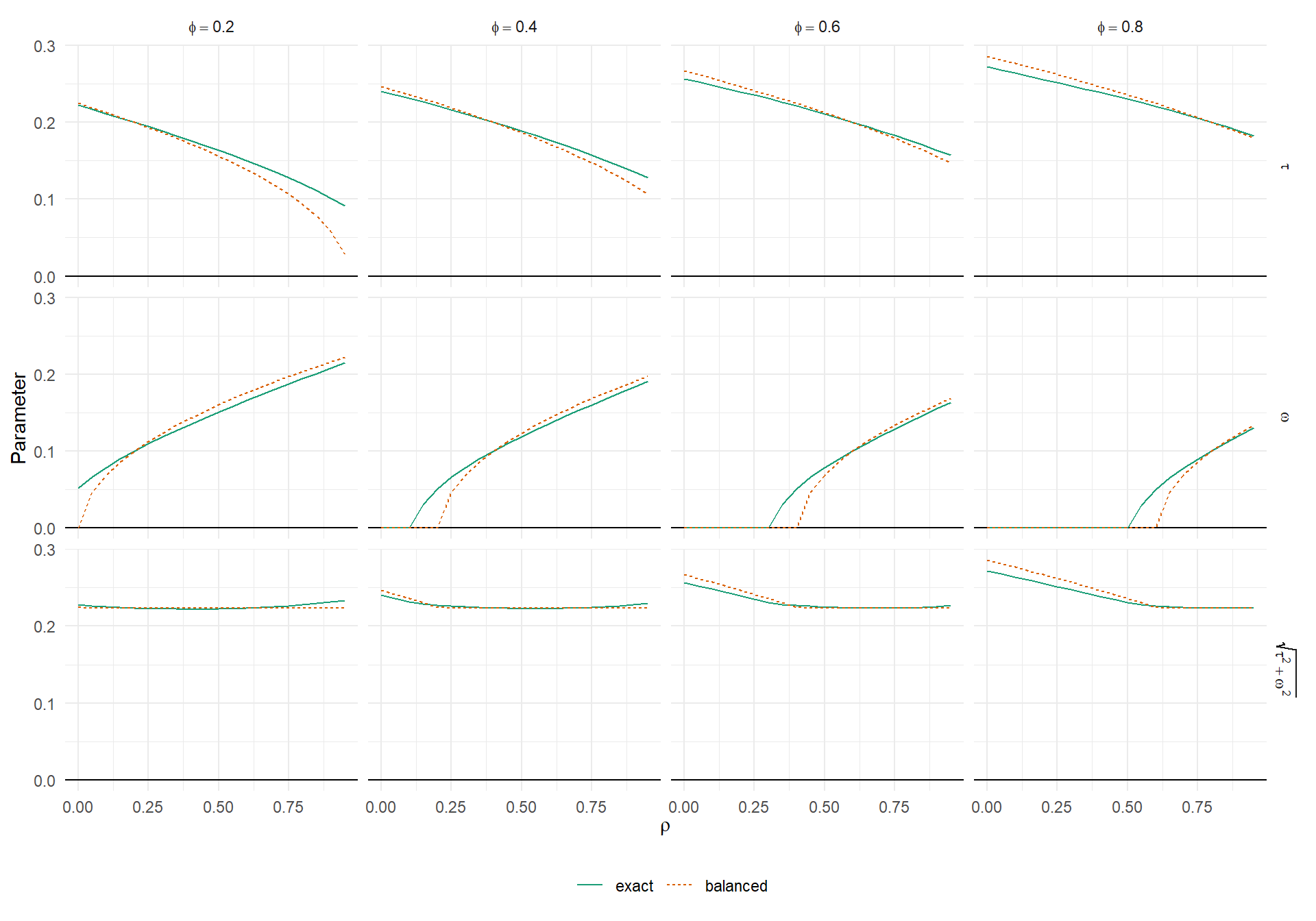
The top row of the figure shows \(\tilde\tau\), the middle row shows \(\tilde\omega\), and the bottom row shows the total SD, for varying levels of assumed correlation \(\rho\). The solid green lines represent the values that actually minimize the KL divergence. The dashed orange lines correspond to the minimizing values assuming complete balance (and using the average value of the \(\sigma_j^2\)’s to evaluate the bias). The “balanced” approximations are fairly close—close enough to use as heuristics, at least—although they’re not perfect. In particular, the balanced approximation becomes discrepant from the real minimizing values when \(\tilde\tau\) or \(\tilde\omega\) gets closer to zero. It’s also notable that the total variance is nearly constant (except when one or the other variance component is zero) and the balanced approximation is quite close to the real minimizing values.
Implications
This post was mostly just to satisfy my own curiosity about how variance components behave in the MLMA and, more broadly, under mis-specified correlated-and-hierarchical effects meta-analysis models. I don’t think the bias formulas have much practical utility because, if you’re concerned about bias due to mis-specified sampling correlations, the first thing to do is try and develop better assumptions about the sampling correlation structure. Still, I think this analysis might be helpful for purposes of gauging how far off from the true your variance component estimates might be. In further work along these lines, it might be useful to examine the consequences of the biased variance component estimates for the efficiency of overall average effect size estimates based on mis-specified CHE models and the accuracy of model-based standard errors and confidence intervals under mis-specification. It would also be important to verify that these approximations provide accurate predictions for the bias of variance component estimates in realistic meta-analytic data (especially with a small or moderate number of studies).
Another implication of this investigation is that imbalance in the data structure seems to matter. When all studies have an equal number of effect sizes and are equally precise, then everything is simpler and more robust to mistaken assumptions about sampling correlation. Variance component estimation matters more for meta-analytic data in which some studies are more precise or contribute more effect size estimates than others. Therefore, further investigations—including simulation studies—of methods for handling dependent effect sizes really need to examine conditions with imbalanced data in order to draw defensible, generalizable conclusions about the robustness or utility of particular methods.
Consequently, \(\phi\) is not identifiable (in the statistical sense) in the completely balanced design.↩︎